Goal - finding team strength with regression¶

There are 3 different regression methods I can think of to find team strength:

I'm going to try method 1 and 3 in this notebook.

Method 1:¶

Our goal is to find each team's strength. One possible way to do it is to create a linear equation for each game:

\begin{equation*} Team_i - Team_j = \Delta {Score} \end{equation*}

Where: \begin{equation*} \Delta {Score} = PointsScored_i - PointsScored_j \end{equation*}

$Team_i$ and $Team_j$ indicate the true strength of teams i and j respectively. Those are the variables we want to find. The $\Delta Score$ is the margin between the two team for the specific game - this is the dependent variable which we know.

It is also possible to separate the linear equation into offensive and defensive strength and thus double the number of unknowns. This is what they do in reference 1.

We need to decide how to treat home court advantage. There are 3 ways I can think of:

Global home court advantage - this means that we add a home court advantage to each of the linear equations. This will be a global variable (i.e. not specific to a team).
Team specific home court advantage - we add a home court variable to each team. In this case we will try and find 2 unknowns for each team (home court and true strength).
Ignore home court advantage

Our linear equation is $\mathbf{y = Ax}$.

y is a vector of game scores: \begin{equation*} \begin{bmatrix} \Delta {Score}_1 \\ ... \\ \Delta {Score}_n \end{bmatrix} \end{equation*}

where n is the number of games played.

x is a vector of the unknown team true strength: \begin{equation*} \begin{bmatrix} Team_1 \\ ... \\ Team_m \end{bmatrix} \end{equation*}

where m is the number of teams.

The trick is how to encode A, which is an nm matrix, so we get the desired equations.
For each row we need to encode A in the following way:
\begin{equation} A_k = \begin{cases} 1 & \text{if i} \\ -1 & \text{if j}\\ 0 & \text{otherwise} \end{cases} \end{equation*}

where i and j indicate teams i and j respectively and k indicates the row number.

Global home court variable¶

If we want to add a global home court advantage we can update our x vector to be: \begin{equation*} \begin{bmatrix} HC \\ Team_1 \\ ... \\ Team_m \end{bmatrix} \end{equation*}

and add a (1st) column to A where each row is 1 if $Team_i$ played home, -1 if $Team_j$ played at home or 0 if the game was at a neutral location.

Method 2:¶

I'll refer you to the link for a detailed explanation.

Method 3:¶

It is very similar to method 1 but in this case we are going to use logistic regression and instead of game margin as the dependent variable we will just use a binary indicator - 1 if $Team_i$ won the game otherwise 0.

We are trying to find the same vector x as before. Our matrix A will also be identical.

To gain a better intuition about what we are trying to optimize, we can look at the resulting probability for $Team_i$ to win a matchup against $Team_j$:

\begin{equation*} p = \frac{1}{1+{e}^{-(Team_i - Team_j)}} \end{equation*}

Let's look at 3 cases:

$Team_i \gg Team_j$, the term in the exponent will be large and negative and we will get $p \approx 1$.
$Team_i \ll Team_j$, the term in the exponent will be large and positive and we will get $p \approx 0$.
$Team_i = Team_j$, we will get 0.5.

We are however, disregarding any win margin in this method as if we are saying that a win is a win regardless of margin.

Regression methodology¶

We are going to try and optimize the team strength from the regular season to predict the results of the NCAA tournament. To do so we are going to try Ridge and Lasson regression and find the best regularization parameter using cross validation.

Data Analysis:¶

In [50]:

import pandas as pd
import matplotlib.pyplot as plt
import glob
import numpy as np
pd.options.display.max_rows = 200
from sklearn.linear_model import Ridge,Lasso,LogisticRegression
from sklearn.metrics import log_loss
from IPython.core.display import display, HTML

display(HTML("<style>.container { width:65% !important; }</style>"))
%matplotlib inline

Load Data¶

This will allow us to easily load the relevant data

In [3]:

files = glob.glob('google-cloud-ncaa-march-madness-2020-division-1-mens-tournament/MDataFiles_Stage1/*')
file_dict = {f.split("\\")[-1].split(".")[0]:f for i,f in enumerate(files)}
for i in file_dict.keys():
    print(i)

Cities
Conferences
MConferenceTourneyGames
MGameCities
MMasseyOrdinals
MNCAATourneyCompactResults
MNCAATourneyDetailedResults
MNCAATourneySeedRoundSlots
MNCAATourneySeeds
MNCAATourneySlots
MRegularSeasonCompactResults
MRegularSeasonDetailedResults
MSeasons
MSecondaryTourneyCompactResults
MSecondaryTourneyTeams
MTeamCoaches
MTeamConferences
MTeams
MTeamSpellings

We want the regular season results:

In [4]:

SeasonResults = pd.read_csv(file_dict['MRegularSeasonCompactResults'])
SeasonResults.head(10)

Out[4]:

	Season	DayNum	WTeamID	WScore	LTeamID	LScore	WLoc
0	1985	20	1228	81	1328	64	N
1	1985	25	1106	77	1354	70	H
2	1985	25	1112	63	1223	56	H
3	1985	25	1165	70	1432	54	H
4	1985	25	1192	86	1447	74	H
5	1985	25	1218	79	1337	78	H
6	1985	25	1228	64	1226	44	N
7	1985	25	1242	58	1268	56	N
8	1985	25	1260	98	1133	80	H
9	1985	25	1305	97	1424	89	H

We will also load the NCAA tournament result.

In [5]:

TourneyCompactResults = pd.read_csv(file_dict['MNCAATourneyCompactResults'])
TourneyCompactResults['TeamID1'] = np.minimum(TourneyCompactResults['WTeamID'],TourneyCompactResults['LTeamID'])
TourneyCompactResults['TeamID2'] = np.maximum(TourneyCompactResults['WTeamID'],TourneyCompactResults['LTeamID'])
TourneyCompactResults['result'] = np.where(TourneyCompactResults['WTeamID']==TourneyCompactResults['TeamID1'],1,0)
#TourneyCompactResults['ID'] = TourneyCompactResults['Season'].astype(str)+ '_' +TourneyCompactResults['TeamID1'].astype(str)+ '_' +TourneyCompactResults['TeamID2'].astype(str)

Regression - Method 1 & 3¶

In [56]:

def team_strength_regression(data,seasons,alpha=0.008,reg_type='Lasso',home=False,days=133,zscore=False):
    """Find the true team strength by adjusting for opponent and score. Computes the strength based on a single season.
    For each game we are trying to solve the following equation: team1_loc + team1 - team2 = team1_points - team2_points.
    Input:
    data - pandas data frame with same structure as the Kaggle NCAA MRegularSeasonCompactResults or MNCAATourneyDetailedResults
    files
    seasons - a list/array of seasons to compute the strength for
    alpha (default = 0.008) - the regularization parameter
    reg_type (default = Lasso) - 'Lasso', 'Ridge' or 'Logistic'
    home (default = False) - if True includes a global home court advanatge variable in the regression
    days (default = 133) - only includes games with DayNum < days. 
    zscore (default = False) - if True computes the zscore for each season
    Example:
    team_strength = team_strength_regression(SeasonResults,np.arange(1985,2020),alpha=0.01,reg_type='Lasso')
    """
    df_list = []
    for s in seasons:
        # get a single season at a time
        SingleSeason = data[(data['Season']==s) & (data['DayNum']<=days)].copy()
        # TeamID1 is always the team with the smaller team ID
        SingleSeason['TeamID1'] = np.minimum(SingleSeason['WTeamID'],SingleSeason['LTeamID'])
        SingleSeason['TeamID2'] = np.maximum(SingleSeason['WTeamID'],SingleSeason['LTeamID'])
        SingleSeason['Score'] = np.where(SingleSeason['WTeamID']==SingleSeason['TeamID1'],
                                         SingleSeason['WScore']-SingleSeason['LScore'],
                                         SingleSeason['LScore']-SingleSeason['WScore'])
        # maps location to number
        SingleSeason['LocN'] = SingleSeason['WLoc'].map({'H':1,'A':-1,'N':0})
        # home court for variable team 1 (1 for home, -1 for away and 0 if neutral)
        SingleSeason['Loc1'] = np.where(SingleSeason['WTeamID']==SingleSeason['TeamID1'],
                                         SingleSeason['LocN'],
                                         -1*SingleSeason['LocN'])
        
        # find all of the unique teams
        unique_teams = pd.concat([SingleSeason['TeamID1'],SingleSeason['TeamID2']],axis=0).unique()
        
        # intialize the A matrix
        if home:
            A = np.zeros((len(SingleSeason),len(unique_teams)+1))
            A[:,-1] = SingleSeason['Loc1']
        else:
            A = np.zeros((len(SingleSeason),len(unique_teams)))
        
        # create a teamID and team index dictionary
        team_dict = dict(zip(unique_teams,np.arange(len(unique_teams))))
        # runs a loop for each game and encodes the matrix A
        for ii,idx in enumerate(zip(SingleSeason['TeamID1'].map(team_dict),SingleSeason['TeamID2'].map(team_dict))):
            A[ii,idx[0]] = 1
            A[ii,idx[1]] = -1
            
        y = SingleSeason['Score'].values
     
        if reg_type == 'Lasso':
            lin = Lasso(alpha=alpha);
        elif reg_type == 'Ridge':
            lin = Ridge(alpha=alpha);
        elif reg_type == 'Logistic':
            lin = LogisticRegression(C=1/alpha,fit_intercept=False,solver='lbfgs',max_iter=500);
            y = np.where(y>0,1,0)
        else:
            print('reg_type is not recognized. Using Lasso.')
            lin = Lasso(alpha=alpha);
            
        lin.fit(A,y);
        
        team_strength = pd.DataFrame(team_dict,index=['team_index']).T.reset_index().rename({'index':'TeamID'},axis=1).drop('team_index',axis=1)
        
        if home:
            if reg_type == 'Logistic':
                team_strength['strength'] = lin.coef_.ravel()[:-1]
                team_strength['home'] = lin.coef_.ravel()[-1]
            else:
                team_strength['strength'] = lin.coef_[:-1]
                team_strength['home'] = lin.coef_[-1]
        else:
            if reg_type == 'Logistic':
                team_strength['strength'] = lin.coef_.ravel()
            else:
                team_strength['strength'] = lin.coef_
        
        if zscore:
            mean_strength = team_strength['strength'].mean()
            std_strength = team_strength['strength'].std()
            team_strength['strength'] = (team_strength['strength'] - mean_strength)/std_strength
            
        team_strength['Season'] = s
        df_list.append(team_strength)
        
    return pd.concat(df_list,ignore_index=True)

Let's try it out. I'll set the regularization to be really low which will be equivalent to Ordinary least squares Linear Regression. I'm also loading the teams data so we can inspect it by name.
I'm using zscore = True - which computes the zscore for every season. This will insure that the results are relative to other teams in the same season. The output units in this case are standard deviation above the mean.

In [36]:

teams = pd.read_csv(file_dict['MTeams'],usecols=['TeamID','TeamName'])
team_strength = team_strength_regression(SeasonResults,
                                         np.arange(1985,2020),
                                         alpha=1e-6,
                                         reg_type='Ridge',
                                         home=True,
                                         zscore=True)
team_strength_with_name = teams.merge(team_strength,on='TeamID')

We can look at the top teams from 1985-2019 season

In [35]:

team_strength_with_name.sort_values(by='strength',ascending=False).head(10)

Out[35]:

	TeamID	TeamName	strength	home	Season
2428	1181	Duke	3.349601	4.348102	1999
2430	1181	Duke	3.141127	4.378684	2001
4432	1246	Kentucky	3.097561	3.184573	2015
9948	1424	UNLV	3.087512	4.383940	1991
6884	1328	Oklahoma	3.044480	4.643256	1988
2427	1181	Duke	3.001867	4.060626	1998
4413	1246	Kentucky	2.983363	3.899327	1996
6505	1314	North Carolina	2.925891	4.074696	2005
3406	1211	Gonzaga	2.891163	3.099425	2019
4414	1246	Kentucky	2.876729	4.327347	1997

In [38]:

team_strength_with_name.to_csv('NCAA_team_strength.csv',index=False)

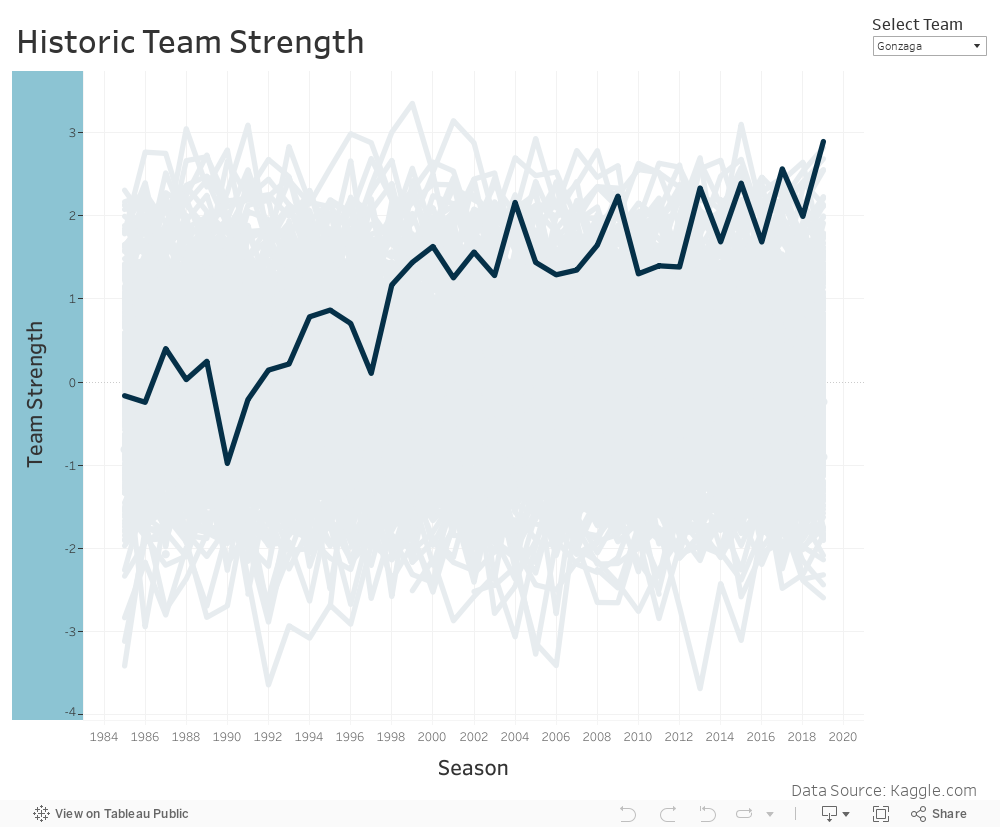
Visualize Results¶

I created a dashboard in Tableau to visualize a teams strength over time:

In [88]:

%%HTML
<div class='tableauPlaceholder' id='viz1588656250429' style='position: relative'><noscript><a href='#'><img alt=' ' src='https:&#47;&#47;public.tableau.com&#47;static&#47;images&#47;NC&#47;NCAAteamstrength&#47;Dashboard&#47;1_rss.png' style='border: none' /></a></noscript><object class='tableauViz'  style='display:none;'><param name='host_url' value='https%3A%2F%2Fpublic.tableau.com%2F' /> <param name='embed_code_version' value='3' /> <param name='site_root' value='' /><param name='name' value='NCAAteamstrength&#47;Dashboard' /><param name='tabs' value='no' /><param name='toolbar' value='yes' /><param name='static_image' value='https:&#47;&#47;public.tableau.com&#47;static&#47;images&#47;NC&#47;NCAAteamstrength&#47;Dashboard&#47;1.png' /> <param name='animate_transition' value='yes' /><param name='display_static_image' value='yes' /><param name='display_spinner' value='yes' /><param name='display_overlay' value='yes' /><param name='display_count' value='yes' /><param name='filter' value='publish=yes' /></object></div>                <script type='text/javascript'>                    var divElement = document.getElementById('viz1588656250429');                    var vizElement = divElement.getElementsByTagName('object')[0];                    if ( divElement.offsetWidth > 800 ) { vizElement.style.width='1000px';vizElement.style.height='827px';} else if ( divElement.offsetWidth > 500 ) { vizElement.style.width='1000px';vizElement.style.height='827px';} else { vizElement.style.width='100%';vizElement.style.height='727px';}                     var scriptElement = document.createElement('script');                    scriptElement.src = 'https://public.tableau.com/javascripts/api/viz_v1.js';                    vizElement.parentNode.insertBefore(scriptElement, vizElement);                </script>

Cross-Validation¶

Im going to try and find the best regularization parameter. The method I'm choosing is to calculate the team strength for different parameters and then run logistic regression on the strength difference between the teams to predict the NCAA tournament results.
I'm going to test it for a few seasons by training the logistic regression on all the seasons before the season at question and then testing the log loss score for that season. This is similar to Time-Series Cross-Validation.

For example:

train for all the seasons between 1985 and 2013 and predict 2014
train for all the seasons between 1985 and 2014 and predict 2015
etc.

I'm going to create a function to hypertune the model

In [76]:

def hypertune_model(reg_type,alphas,homes,zscores):
    # Define predictive model for the trounament with low regularization parameter 
    lr = LogisticRegression(solver='lbfgs',C=1000000,random_state=0,max_iter=1500)

    all_scores = []
    for zscore in zscores:
        for home in homes:
            for alpha in alphas:  
                # get team strength
                team_strength = team_strength_regression(SeasonResults,
                                                         np.arange(1985,2020),
                                                         alpha=alpha,
                                                         reg_type=reg_type,
                                                         home=home,
                                                         zscore=zscore)

                # join to tournament data
                TourneyResults = (TourneyCompactResults
                                         .merge(team_strength,left_on=['Season','TeamID1'],right_on=['Season','TeamID'],how='left')
                                         .drop('TeamID',axis=1)
                                         .merge(team_strength,left_on=['Season','TeamID2'],right_on=['Season','TeamID'],how='left')
                                         .drop('TeamID',axis=1)
                                        ).copy()

                TourneyResults['strength_diff'] = TourneyResults['strength_x'] - TourneyResults['strength_y']

                cols = ['strength_diff']

                # define model variables
                X = TourneyResults.loc[:,cols]
                y = TourneyResults[['result']].values.ravel()

                # run cross validation
                scores = np.zeros((5,1))
                for ii,s in enumerate(range(2014,2019)):
                    idxTrain = (TourneyResults['Season'] < s) 
                    idxTest = (TourneyResults['Season'] == s)
                    # fit all models
                    lr.fit(X.loc[idxTrain],y[idxTrain])

                    ypred_lr = lr.predict_proba(X.loc[idxTest])

                    scores[ii,0] = log_loss(y[idxTest],ypred_lr[:,1])

                all_scores.append([zscore,home,alpha,np.mean(scores),np.std(scores)])

    return pd.DataFrame(all_scores,columns=['zscore','home','alpha','log_loss_mean','log_loss_std'])

Ridge Regression¶

I'm going to try a grid search on a few parameters to see which ones yields the best results on the test data

In [62]:

all_scores_df = hypertune_model('Ridge',[0.001,0.01,0.1,1,10,100],[False,True],[False,True])

In [63]:

# use this to highlight the minimum value - https://pandas.pydata.org/pandas-docs/stable/user_guide/style.html
def highlight_min(s):
    '''
    highlight the maximum in a Series yellow.
    '''
    is_min = s == s.min()
    return ['background-color: yellow' if v else '' for v in is_min]

In [64]:

all_scores_df
all_scores_df.style.apply(highlight_min,subset=['log_loss_mean'])

Out[64]:

	zscore	home	alpha	log_loss_mean	log_loss_std
0	False	False	0.001	0.549705	0.0414636
1	False	False	0.01	0.549692	0.0414647
2	False	False	0.1	0.549569	0.0414741
3	False	False	1	0.548619	0.0414582
4	False	False	10	0.551865	0.0387321
5	False	False	100	0.588166	0.0323496
6	False	True	0.001	0.549162	0.0399869
7	False	True	0.01	0.549155	0.0399835
8	False	True	0.1	0.549089	0.0399488
9	False	True	1	0.548761	0.039533
10	False	True	10	0.558743	0.0353229
11	False	True	100	0.602036	0.0289713
12	True	False	0.001	0.550154	0.042132
13	True	False	0.01	0.550139	0.0421293
14	True	False	0.1	0.549999	0.0421009
15	True	False	1	0.5489	0.0417868
16	True	False	10	0.551654	0.0383788
17	True	False	100	0.587731	0.0317663
18	True	True	0.001	0.549818	0.0407387
19	True	True	0.01	0.549809	0.040733
20	True	True	0.1	0.549725	0.0406757
21	True	True	1	0.549242	0.0400891
22	True	True	10	0.558724	0.0354915
23	True	True	100	0.601817	0.0287516

Lasso Regression¶

In [73]:

all_scores_df2 = hypertune_model('Lasso',[0.001,0.002,0.004,0.008,0.016],[False,True],[False,True])

In [74]:

all_scores_df2
all_scores_df2.style.apply(highlight_min,subset=['log_loss_mean'])

Out[74]:

	zscore	home	alpha	log_loss_mean	log_loss_std
0	False	False	0.001	0.549031	0.0416238
1	False	False	0.002	0.548442	0.0416927
2	False	False	0.004	0.547319	0.0416859
3	False	False	0.008	0.546306	0.0423778
4	False	False	0.016	0.551118	0.0419727
5	False	True	0.001	0.548509	0.0399868
6	False	True	0.002	0.548018	0.0399782
7	False	True	0.004	0.547927	0.0400741
8	False	True	0.008	0.550062	0.0407204
9	False	True	0.016	0.56028	0.0397972
10	True	False	0.001	0.549466	0.0423643
11	True	False	0.002	0.548861	0.0425223
12	True	False	0.004	0.54769	0.0426924
13	True	False	0.008	0.546565	0.0437606
14	True	False	0.016	0.551263	0.0444069
15	True	True	0.001	0.549166	0.0408685
16	True	True	0.002	0.548661	0.040987
17	True	True	0.004	0.548558	0.041361
18	True	True	0.008	0.550653	0.0426055
19	True	True	0.016	0.56081	0.0429843

The best result so far is the Lasso regression without zscore and home advantage variable and with a 0.008 regularization parameter.

Logistic Regression¶

In [77]:

 all_scores_df3 = hypertune_model('Logistic',[0.001,0.01,0.1,1,10,100],[False,True],[False,True])

In [78]:

all_scores_df3
all_scores_df3.style.apply(highlight_min,subset=['log_loss_mean'])

Out[78]:

	zscore	home	alpha	log_loss_mean	log_loss_std
0	False	False	0.001	0.578268	0.0334135
1	False	False	0.01	0.570982	0.0308209
2	False	False	0.1	0.565409	0.0290306
3	False	False	1	0.568223	0.0207406
4	False	False	10	0.607005	0.00964444
5	False	False	100	0.633217	0.00844086
6	False	True	0.001	0.581161	0.0319527
7	False	True	0.01	0.573997	0.0278307
8	False	True	0.1	0.569932	0.0249388
9	False	True	1	0.583728	0.0160858
10	False	True	10	0.631672	0.0070408
11	False	True	100	0.650116	0.00597512
12	True	False	0.001	0.57845	0.03326
13	True	False	0.01	0.571325	0.0305801
14	True	False	0.1	0.565462	0.0287155
15	True	False	1	0.567926	0.0204353
16	True	False	10	0.606475	0.00965828
17	True	False	100	0.632403	0.00843415
18	True	True	0.001	0.582715	0.0328544
19	True	True	0.01	0.575477	0.0282869
20	True	True	0.1	0.570783	0.0250404
21	True	True	1	0.583856	0.0159188
22	True	True	10	0.631249	0.00711013
23	True	True	100	0.649327	0.00607005

This method is not as good. Not surprising given the fact that we reduced the game result to a binary variable on purpose.

Compare to other ranking methods¶

Let's see how many tournament games it predicts correctly if we choose the higher rank team to win.

I'm going to call my ranking method SHAr

Note: the regression methods I hypertunned used the data we are checking which gives an unfair advantage. An apple to apples comparison would be to tune the regression on earlier data and test all the methods on the last few years. The disadvantage of that method is that there is much less data to compare outcomes.

In [79]:

ranking = pd.read_csv(file_dict['MMasseyOrdinals'])
rank_methods = ['COL','DOL','MOR','POM','RTH','SAG','WLK','WOL']
team_rank = (ranking[(ranking['RankingDayNum']==133)&(ranking['SystemName'].isin(rank_methods))]
             .groupby(['Season','TeamID','SystemName'])['OrdinalRank']
             .mean()
             .unstack(2)
             .reset_index()
            )

In [82]:

# TourneyCompactResults = pd.read_csv(file_dict['MNCAATourneyCompactResults'])

team_strength = team_strength_regression(SeasonResults,
                                         np.arange(1985,2020),
                                         alpha=0.008,
                                         reg_type='Lasso',
                                         home=False,
                                         zscore=False)

data = team_rank.merge(team_strength,on=['Season','TeamID'],how='left')
    

TourneyResults = (TourneyCompactResults
                         .merge(data,left_on=['Season','WTeamID'],right_on=['Season','TeamID'],how='left')
                         .drop('TeamID',axis=1)
                         .merge(data,left_on=['Season','LTeamID'],right_on=['Season','TeamID'],how='left')
                         .drop('TeamID',axis=1)
                        ).copy()

rdata = TourneyResults[TourneyResults['Season']>2002].copy()
rdata['POMr'] = np.where(rdata['POM_y']>rdata['POM_x'],1,0)
rdata['SAGr'] = np.where(rdata['SAG_y']>rdata['SAG_x'],1,0)
rdata['COLr'] = np.where(rdata['COL_y']>rdata['COL_x'],1,0)
rdata['DOLr'] = np.where(rdata['DOL_y']>rdata['DOL_x'],1,0)
rdata['MORr'] = np.where(rdata['MOR_y']>rdata['MOR_x'],1,0)
rdata['RTHr'] = np.where(rdata['RTH_y']>rdata['RTH_x'],1,0)
rdata['WLKr'] = np.where(rdata['WLK_y']>rdata['WLK_x'],1,0)
rdata['WOLr'] = np.where(rdata['WOL_y']>rdata['WOL_x'],1,0)
rdata['SHAr'] = np.where(rdata['strength_x']>rdata['strength_y'],1,0)
g = rdata.groupby('Season')[['POMr','SAGr','COLr','DOLr','MORr','RTHr','WLKr','WOLr','SHAr']].mean()
rank_summary = pd.DataFrame(g.mean(),columns=['PCT_CORRECT'])
rank_summary.sort_values(by='PCT_CORRECT',ascending=False)

Out[82]:

	PCT_CORRECT
SHAr	0.716967
POMr	0.715170
MORr	0.713414
SAGr	0.712371
DOLr	0.707817
WLKr	0.707103
WOLr	0.707062
RTHr	0.706102
COLr	0.701589

Method by Tournament round

In [87]:

# use this to highlight the minimum value - https://pandas.pydata.org/pandas-docs/stable/user_guide/style.html
def highlight_max(s):
    '''
    highlight the maximum in a Series yellow.
    '''
    is_max = s == s.max()
    return ['background-color: yellow' if v else '' for v in is_max]

round_dict = {136:'1: 1st',
              137:'1: 1st',
              138:'2: 2nd',
              139:'2: 2nd',
              143:'3: S16',
              144:'3: S16',
              145:'4: E8',
              146:'4: E8',
              152:'5: F4',
              154:'6: CG'}

rdata['Round'] = rdata['DayNum'].map(round_dict)
round_agg = (rdata[(rdata['Season']<=2019)&(rdata['DayNum']>=136)]
             .groupby('Round')[['POMr','SAGr','COLr','DOLr','MORr','RTHr','WLKr','WOLr','SHAr']]
             .mean()
            )

round_agg.style.apply(highlight_max,axis=1)

Out[87]:

	POMr	SAGr	COLr	DOLr	MORr	RTHr	WLKr	WOLr	SHAr
Round
1: 1st	0.759191	0.744485	0.740809	0.742647	0.748162	0.748162	0.746324	0.744485	0.746324
2: 2nd	0.724265	0.746324	0.724265	0.724265	0.716912	0.735294	0.746324	0.720588	0.735294
3: S16	0.669118	0.698529	0.683824	0.676471	0.676471	0.676471	0.691176	0.669118	0.698529
4: E8	0.529412	0.5	0.485294	0.485294	0.544118	0.485294	0.441176	0.529412	0.529412
5: F4	0.647059	0.617647	0.676471	0.735294	0.647059	0.647059	0.617647	0.617647	0.676471
6: CG	0.647059	0.588235	0.529412	0.588235	0.705882	0.529412	0.529412	0.764706	0.764706

Is my ranking method better at predicting the NCAA tournament compared to other ranking methods?
It is hard to tell because I tunned the regularization parameter on the same data that we are predicting. So I'm probably overfitting the data. If this results hold up over the next few years without modifying the regression parameters then maybe I can claim that.

In [ ]:

NCAA Team Strength